A Guide To in silico Drug Design.
Read about the amazing advancements using in silico
Published online:
2014 Jan. doi: 10.1124/pr.112.007336
PMID:
What is this article about:
in silico Drug Design, Structure-Based Drug Design, Computer Aided Drug Design, Drug Discovery.
Editors:
Gregory Sliwoski, Sandeepkumar Kothiwale, Jens Meiler, and Edward W. Lowe, Jr.
Associate Editor:
Eric L. Barker
Stages of Drug Discovery, Stages of Drug Development, Protein Structure Prediction Tools.
Abstract of in silico Drug Design
The drug discovery process is a rocky path that is full of challenges, with the result that very few candidates progress from hit compound to a commercially available product, often due to factors, such as poor binding affinity, off-target effects, or physicochemical properties, such as solubility or stability. This process is further complicated by high research and development costs and time requirements. It is thus important to optimise every step of the process in order to maximise the chances of success. As a result of the recent advancements in computer power and technology, computer-aided drug design (CADD) has become an integral part of modern drug discovery to guide and accelerate the process. In this review, we present an overview of the important CADD methods and applications, such as in silico structure prediction, refinement, modelling and target validation, that are commonly used in this area.
Introduction: in silico Drug Discovery and Development
New drugs with better efficacy and reduced toxicity are always in high demand, however the process of drug discovery and development is costly and time consuming and presents a number of challenges. The pitfalls of target validation and hit identification aside, a high failure rate is often observed in clinical trials due to poor pharmacokinetics, poor efficacy, and high toxicity [1,2]. A study conducted by Wong et al. that analysed 406,038 trials from January 2000 to October 2015 showed that the probability of success for all drugs (marketed and in development) was only 13.8% [3]. In 2016, DiMasi and colleagues [4] estimated a research and development (R&D) cost for a new drug of USD $2.8 billion based upon data for 106 randomly selected new drugs developed by 10 pharmaceutical companies. The average time taken from synthesis to first human testing was estimated to be approximately 2.6 years (31.2 months) and cost approximately USD $430 million, and from the start of a clinical testing to submission with the FDA was 6 to 7 years (80.8 months). In comparison to a study conducted by the same author in 2003, the R&D cost for a new drug had increased drastically by more than two-fold (from USD $1.2 billion) [5]. A possible reason for the increase in R&D cost is that regulators, such as the FDA have become more risk averse, tightening safety requirements, leading to higher failure rates in trials and increased costs for drug development. It is therefore important to optimise every aspect of the R&D process in order to maximise the chances of success.
The process of drug discovery starts with target identification, followed by target validation, hit discovery, lead optimisation, and preclinical/clinical development. If successful, a drug candidate progresses to the development stage, where it passes through different phases of clinical trials and eventually submission for approval to launch on the market (Figure 1) [6].
Stages of Drug Discovery and Development.
Briefly, drug targets can be identified using methods, such as data-mining [7], phenotype screening [8,9], and bioinformatics (e.g., epigenetic, genomic, transcriptomic, and proteomic methods) [10]. Potential targets must then be validated to determine whether they are rate limiting for the disease’s progression or induction. Establishing a strong link between the target and disease builds up confidence in the scientific hypothesis and thus greater success and efficiency in later stages of the drug discovery process [11,12].
Once the targets are identified and validated, compound screening assays are carried out to discover novel hit compounds (hit-to-lead). There are various strategies that can be used in this screening, involving physical methods, such as mass spectrometry [13], fragment screening [14,15], nuclear magnetic resonance (NMR) screening [16], DNA encoded chemical libraries [17], high throughput screening (HTS) (such as protein or cells) [18] or in silico methods, such as virtual screening (VS) [19].
After hit compounds are identified, properties, such as absorption, distribution, metabolism, excretion (ADME), and toxicity should be considered and optimised early in the drug discovery process. Unfavourable pharmacokinetic and toxicity profile of a drug candidate is one of the hurdles that often leads to failure in the clinical trials [20].
Although physical and computational screening techniques are distinct in nature, they are often integrated in the drug discovery process to complement each other and maximise the potential of the screening results [21].
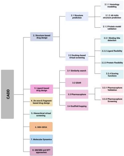
Computer-aided drug design (CADD) utilises this information and knowledge to screen for novel drug candidates. With the advancement in technology and computer power in recent years, CADD has proven to be a tool that reduces the time and resources required in the drug discovery pipeline. The aim of this review is to give an overview of the various in silico techniques that are used in the drug discovery process (Figure 2).

Various in silico techniques used in the drug design and discovery process discussed in this review. (Abbreviations: CADD: computer-aided drug design; DFT: density functional theory; MM: molecular mechanical; MM-GBSA: molecular mechanics with generalised Born and surface area; QM: quantum mechanical; QSAR: quantitative structure activity relationship).
2. Structure-Based Drug Design
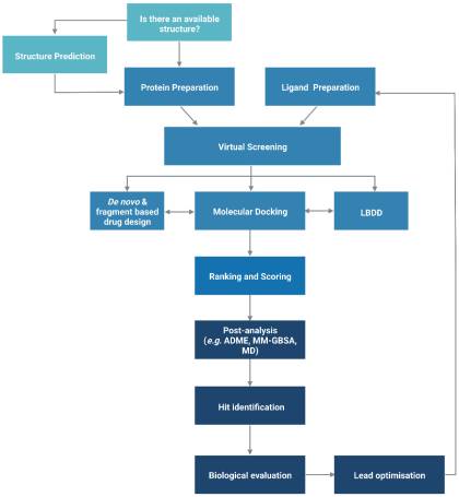
The functionality of a protein is dependent upon its structure, and structure-based drug design (SBDD) relies on the 3D structural information of the target protein, which can be acquired from experimental methods, such as X-ray crystallography, NMR spectroscopy and cryo-electron microscopy (cryo-EM). The aim of SBDD is to predict the Gibbs free energy of binding (ΔGbind), the binding affinity of ligands to the binding site, by simulating the interactions between them. Some examples of SBDD include molecular dynamics (MD) simulations [22], molecular docking [23], fragment-based docking [24], and de novo drug design [25]. Figure 3 describes a general workflow of molecular docking that will be discussed in greater detail.

General workflow of molecular docking. The process begins with the preparation of the protein structure and ligand database separately, followed by molecular docking in which the ligands were ranked based on their binding pose and predicted binding affinity. (Abbreviations: LBDD: Ligand-based drug design; ADME: absorption, distribution, metabolism and excretion; MD: molecular dynamics; MM-GBSA: molecular mechanics with generalised Born and surface area).
2.1. Protein Structure Prediction
The advancements in sequencing technology led to a steep increase in recorded genetic information thus rapidly widening the gap between the amounts of sequence and structural data available. As of May 2022, the UniprotKB/TrEMBL database contained over 231 million sequence entries, yet there are only approximate 193,000 structures recorded in the Protein Data Bank (PDB) [26,27]. To model the structures of those proteins where structural data is not available, homology (comparative) modelling or ab initio methods can be used.
2.1.1. Homology Modelling
Homology modelling involves predicting the structure of a protein by aligning its sequence to a homologous protein that serves as a template for the construction of the model. The process can be broken down into three steps: (1) template identification, (2) sequence-template alignment, and (3) model construction.
Firstly, the protein sequence is obtained, either experimentally or from databases, such as the Universal Protein Resource (UniProt) [28], and this is followed by identifying modelling templates that have high sequence similarity and resolution by performing a BLAST [29] search against the Protein Data Bank [30]. PSI-BLAST [29] uses profile-based methods to identify patterns of residue conservation, which can be more useful and accurate than simply comparing raw sequences, as protein functions are predominately determined by the structural arrangement rather than the amino acid sequence. One of the biggest limitations of homology modelling is that it relies heavily upon the availabilities of suitable templates and accurate sequence alignment. A high sequence identity between the query protein and the template normally gives greater confidence in the homology model. Generally, a minimum of 30% sequence identity is considered to be a threshold for successful homology modelling, as approximately 20% of the residues are expected to be misaligned for sequence identities below 30%, leading to poor homology models. Alignment errors are less frequent when the sequence identity is above 40%, where approximately 90% of the main-chain atoms are likely to be modelled with a root-mean-square deviation (RMSD) of ~1 Å, and the majority of the structural differences occur at loops and in side-chain orientations [31].
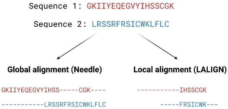
Pairwise alignment methods are used when comparing two sequences and they are generally divided into two categories—global and local alignment (Figure 4). Global alignment aims to align the entire sequences and are most useful when sequences are closely related or of similar lengths. Tools such as EMBOSS Needle [32] and EMBOSS Stretcher [32] use the Needleman–Wunsch algorithm [33] to perform global alignment. In comparison to using a somewhat brute-force approach, the Needleman–Wunsch algorithm uses dynamic programming to find the best alignment by reducing the number of possible alignments that need to be considered and guarantees to find the best alignment. Dynamic programming aims to break a larger problem (the entire sequence) into smaller problems which are then solved optimally. The solutions to these smaller problems are then used to construct an optimal solution to the original problem [34]. The Needleman–Wunsch algorithm first builds a matrix that is subjected to a gap penalty (negative scores in first row and column), and the matrix is used to assign a score to every possible alignment (usually positive score for match, no score or penalty for mismatch and gaps). Once the cells in the matrix are filled in, traceback starts from the lower right towards the top left of the matrix to find the best alignment with the highest score.

Example of global and local alignment using Needle [32] and LALIGN [32]. Global alignment aims to find the best alignment across the two entire length of sequences. Local alignment finds regions of high similarity in parts of the sequences.
Select Link Below To Continue Reading A Guide To in silico Design
Start Your Own Alphaperrin Computational™ Lab Environment
Read the full Publication on PubMed.com

Discovering. Improving.
Drug Design Perfected.
Quick LInks
A Guide To in silico Drug Design
Computational Methods in Drug Discovery
P: 910.756.6106
F: 279.300.3241